Background: Undergraduate
Undergraduate in Psychology
- Statistics
- Experiment Design
- Cognitive Theory
- Neurology
- Humans

Background: PhD
- "Ah, statistics, everything is black and white!
- "There's always an answer"
- "data in, answer out"

Background: PhD
- Data is really messy
- Missing values are frustrating
- How to Explore data?

(My personal) motivation
Focus on building a bridge across a river. Less focus on how it is built, and the tools used.

All of Australia
...And New Zealand
And the rest?
And the rest?


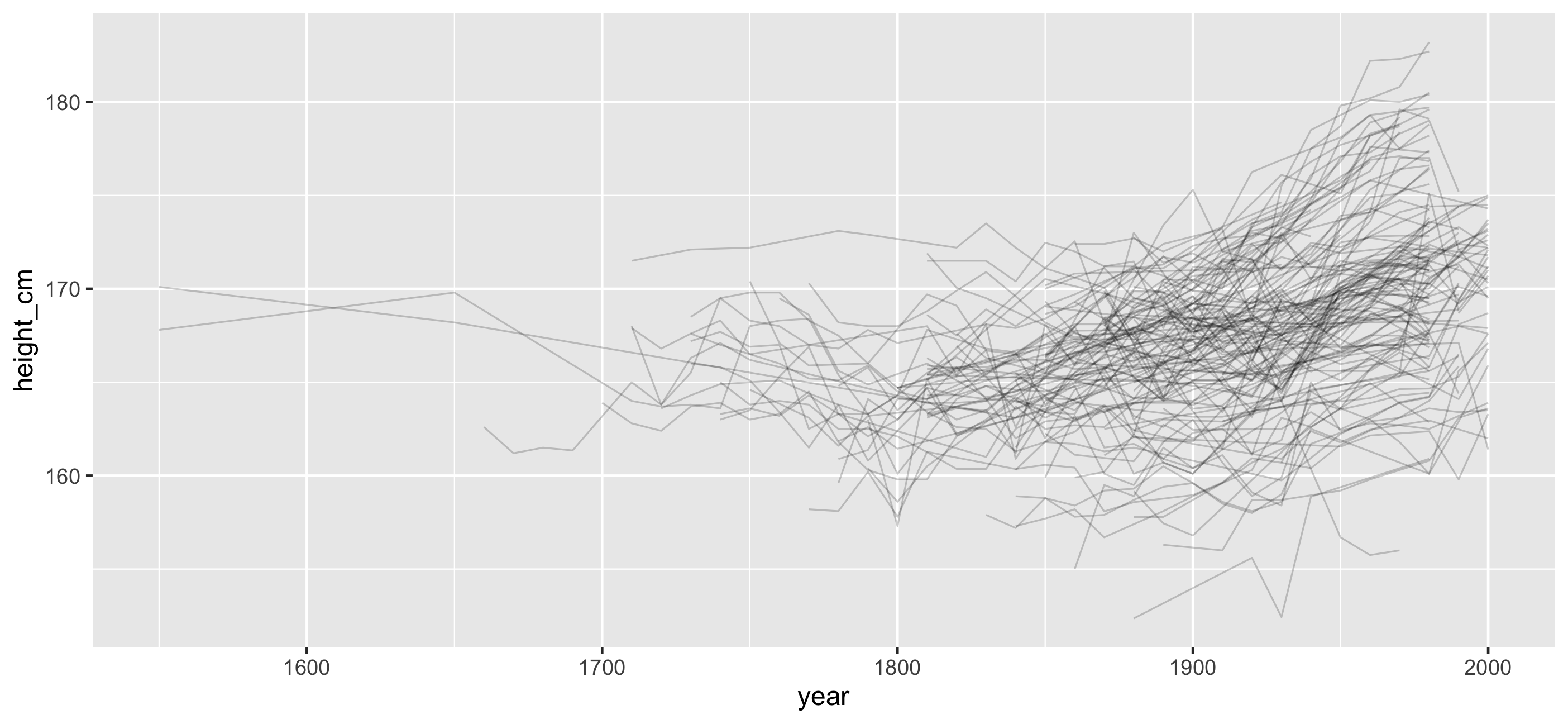
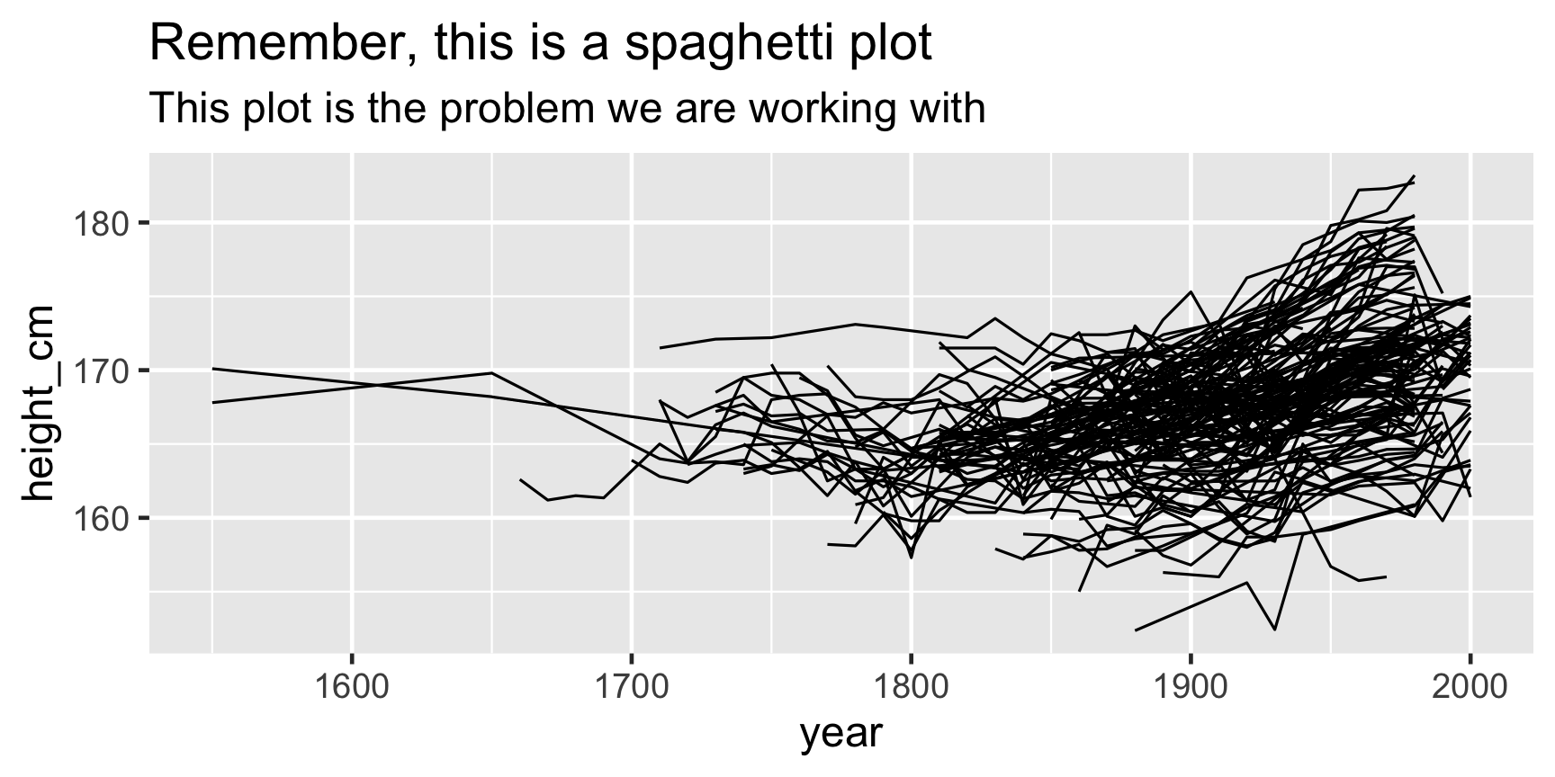
Problems:
- Overplotting
- We don't see the individuals
- We could look at 144 individual plots, but this doesn't help.

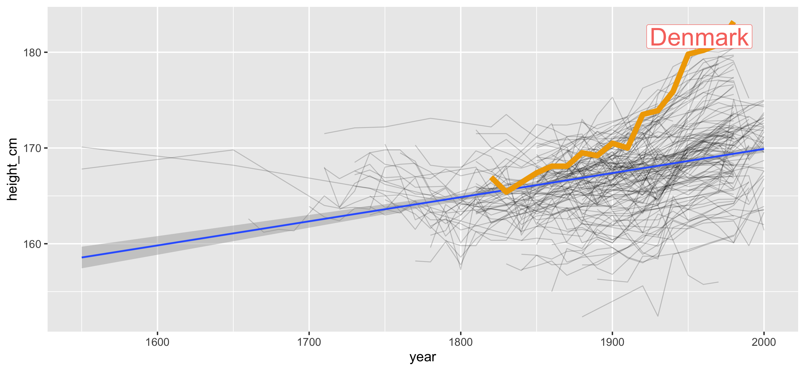
Answers: Transparency?
Answers: Transparency + a model?
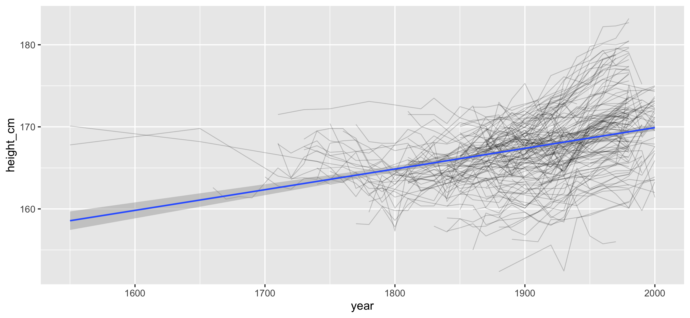
But we forget about the individuals

Introducing brolgar: brolgar.njtierney.com
- browsing
- over
- longitudinal data
- graphically, and
- analytically, in
- r
Longitudinal data as a time series 
heights <- as_tsibble(heights, index = year, key = country, regular = FALSE)- index: Your time variable
- key: Variable(s) defining individual groups (or series)
1. + 2. determine distinct rows in a tsibble.
(From Earo Wang's talk: Melt the clock)
Longitudinal data as a time series
Key Concepts:
Record important time series information once, and use it many times in other places
- We add information about index + key:
- Index = Year
- Key = Country
Problem #1: How do I look at some of the data?
Look at only a sample of the data:

Sample n rows with sample_n()
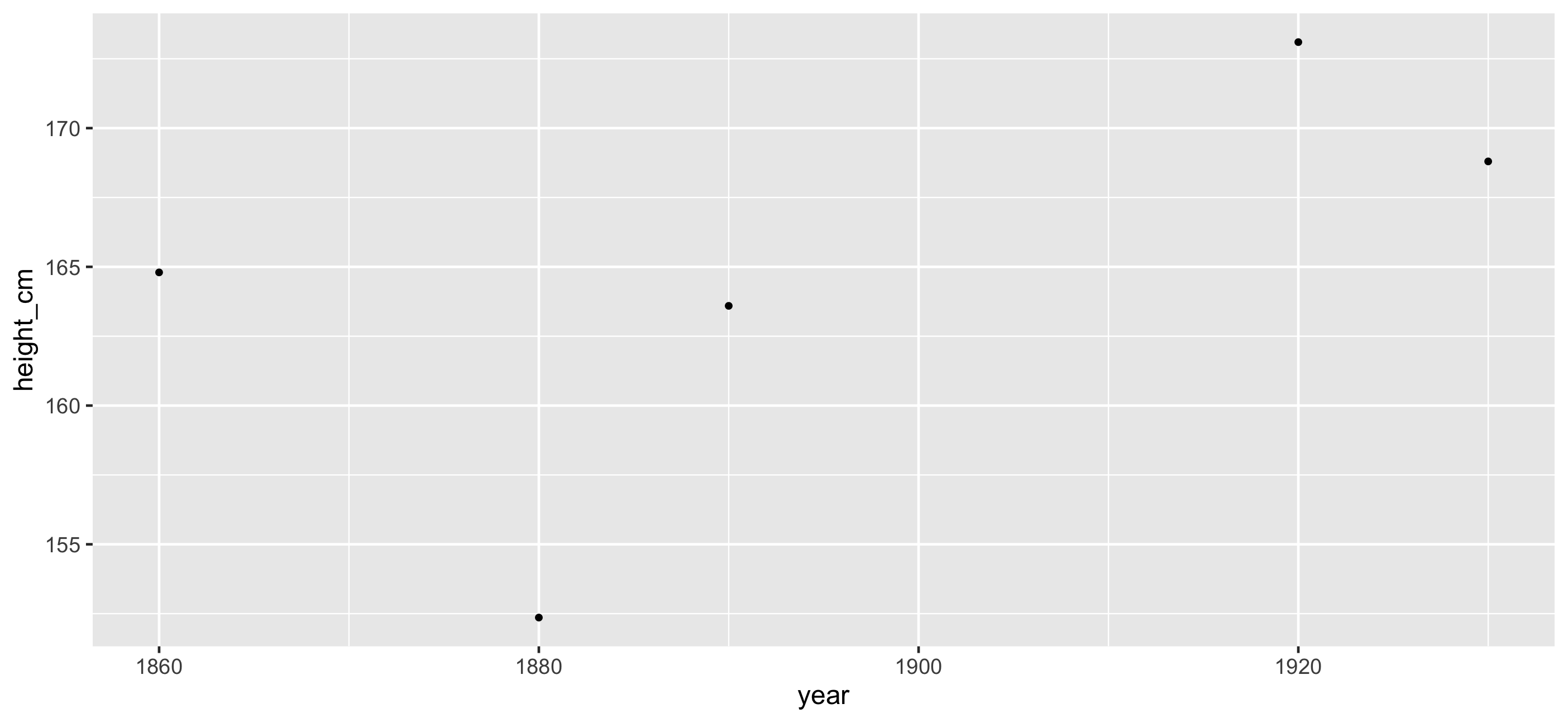
sample_n_keys() to sample ... keys
Portion out your spaghetti! 🍝 🍝 🍝 🍝

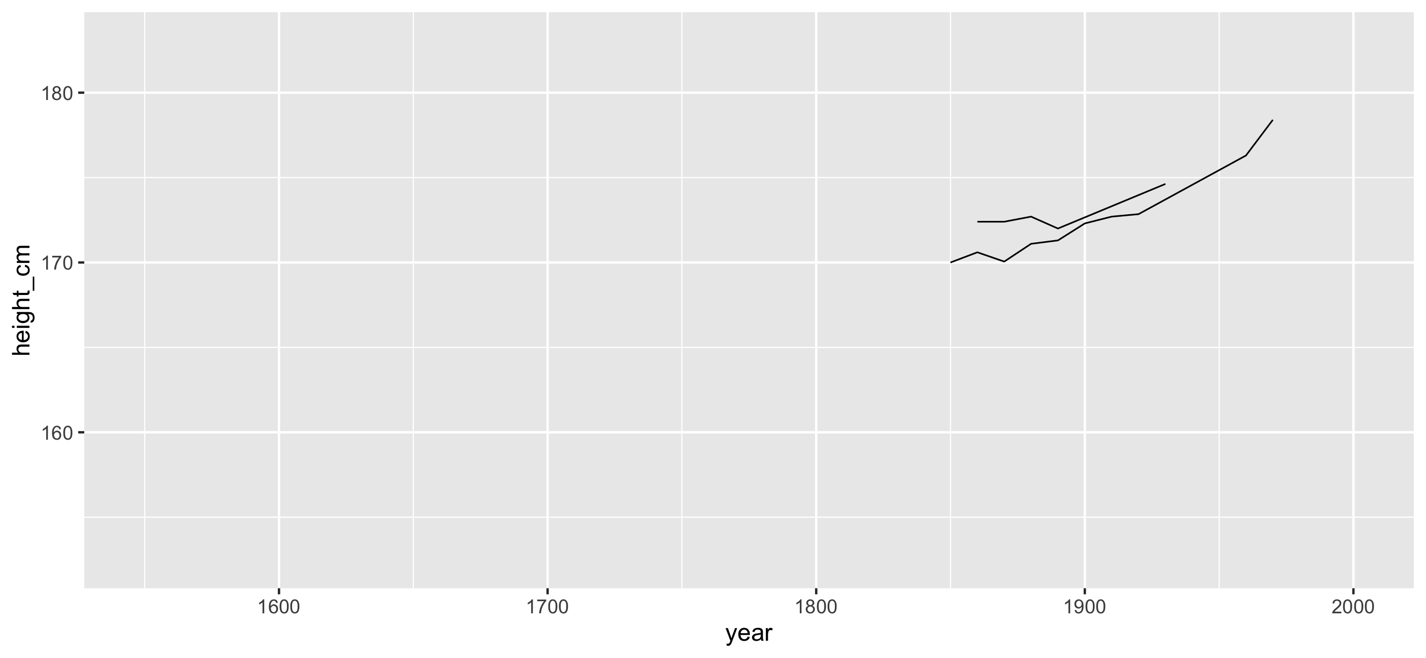
Look at one set of subsamples 🍝

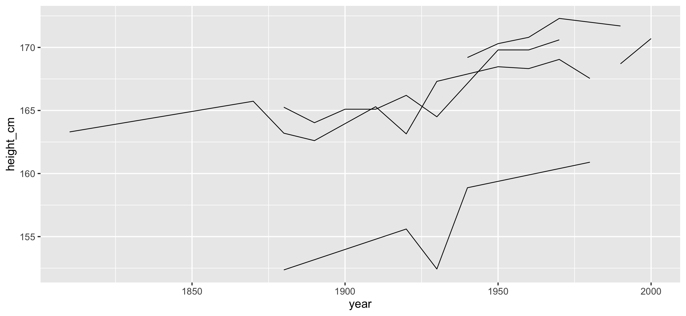
Look at many subsamples 🍝 🍝
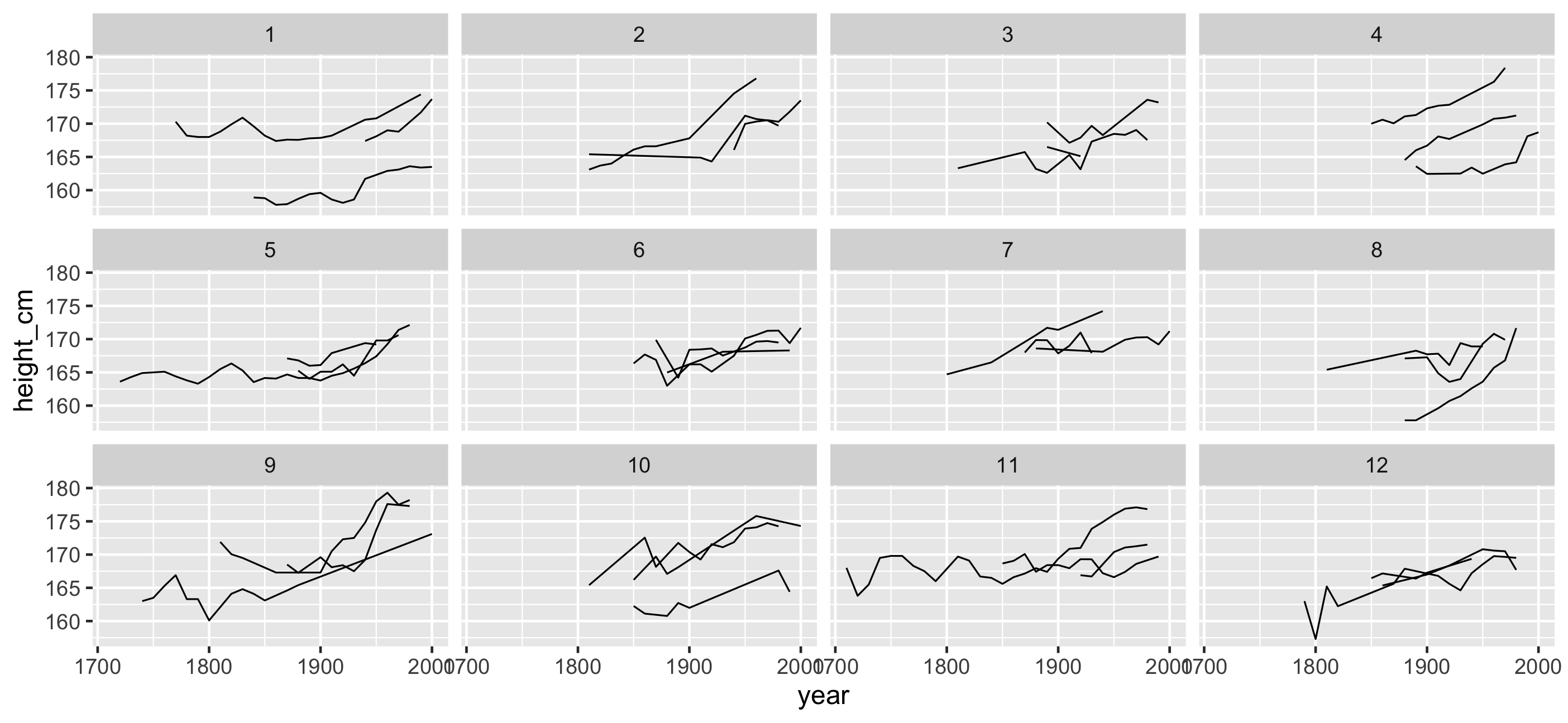

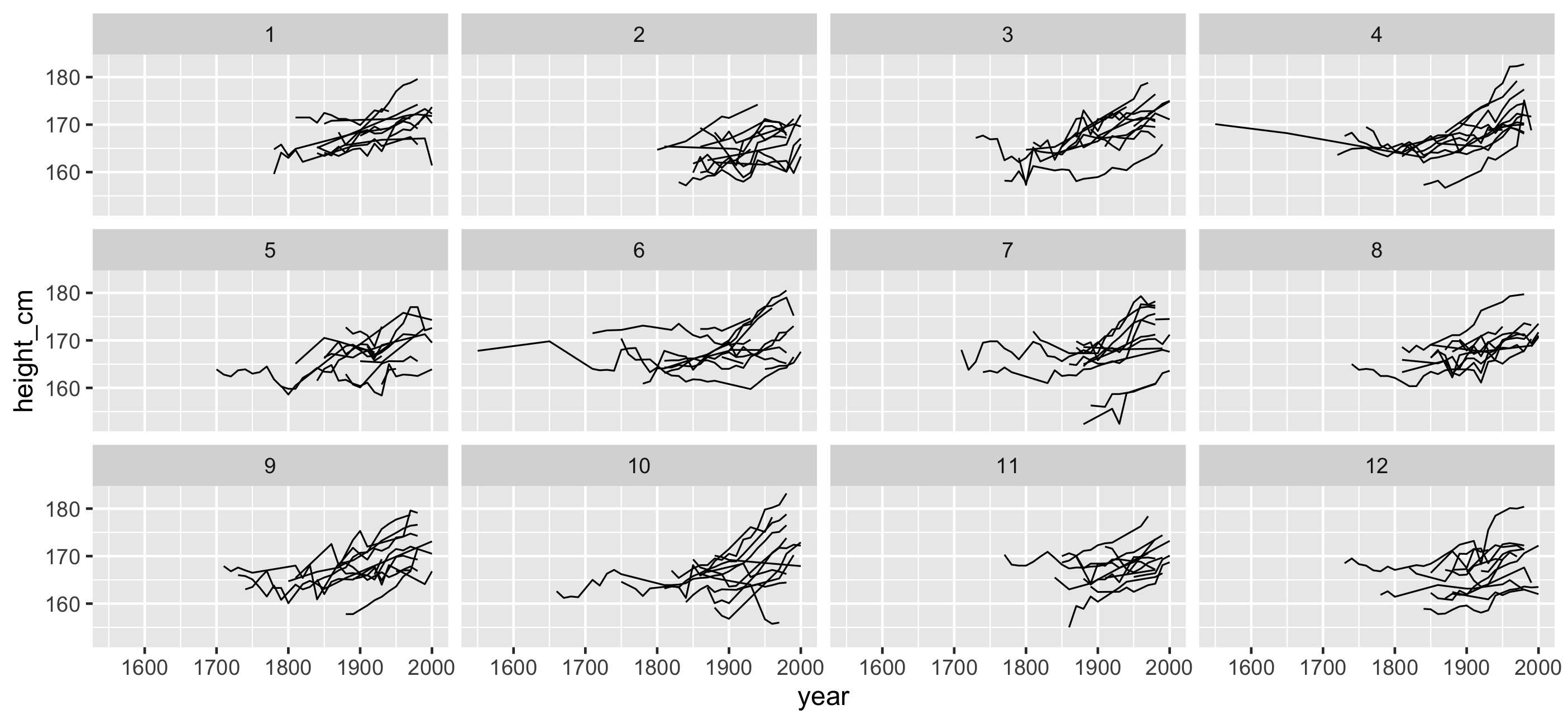
facet_sample(): See more individuals
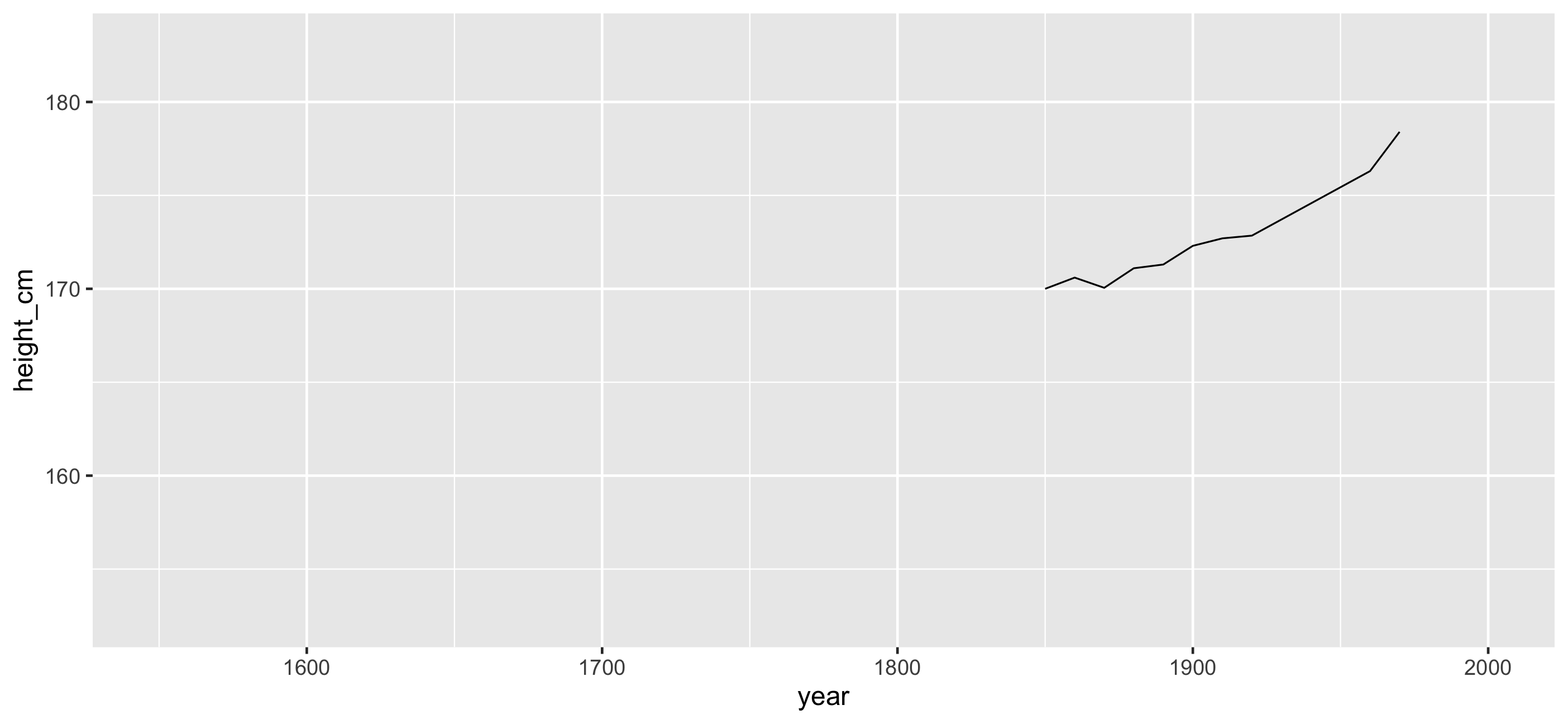
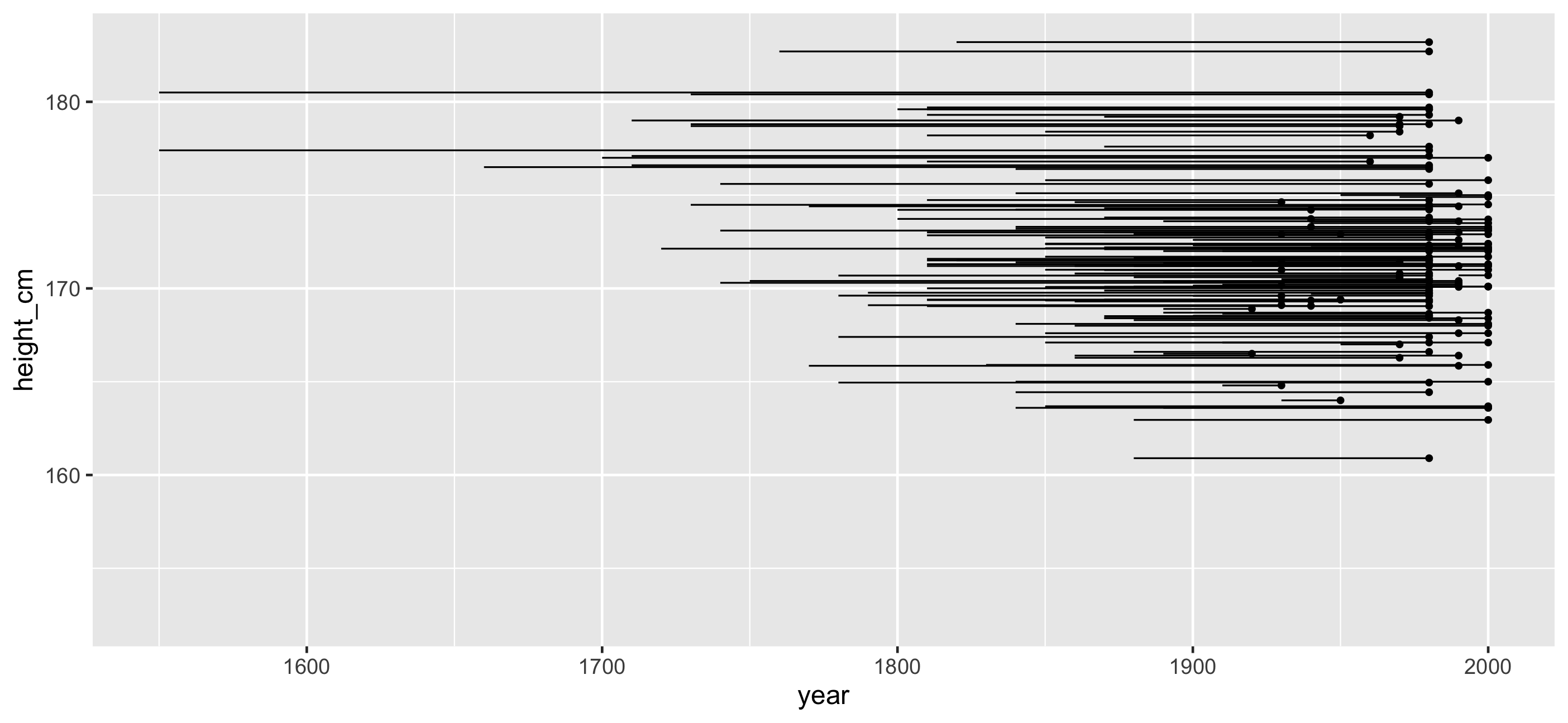
ggplot(heights, aes(x = year, y = height_cm, group = country)) + geom_line()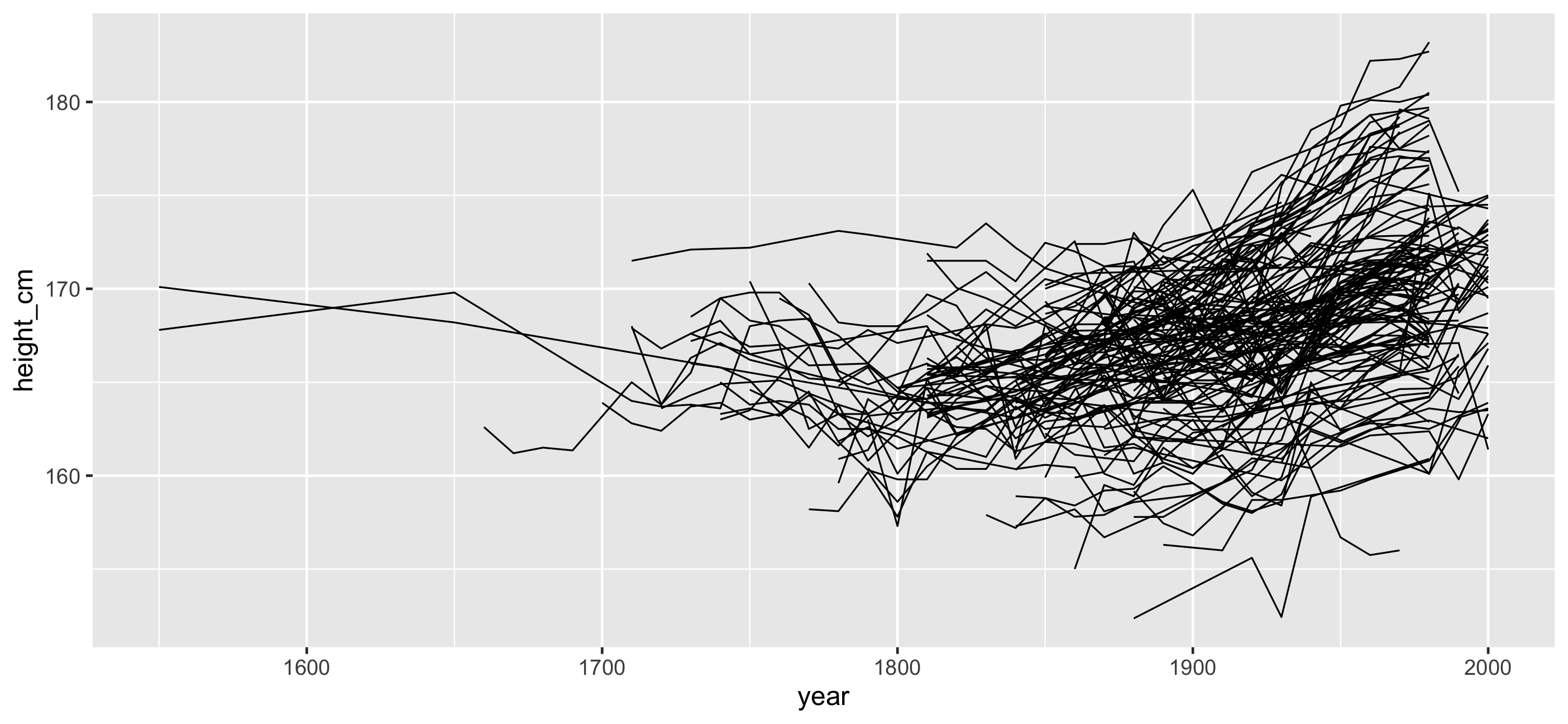
facet_sample(): See more individuals
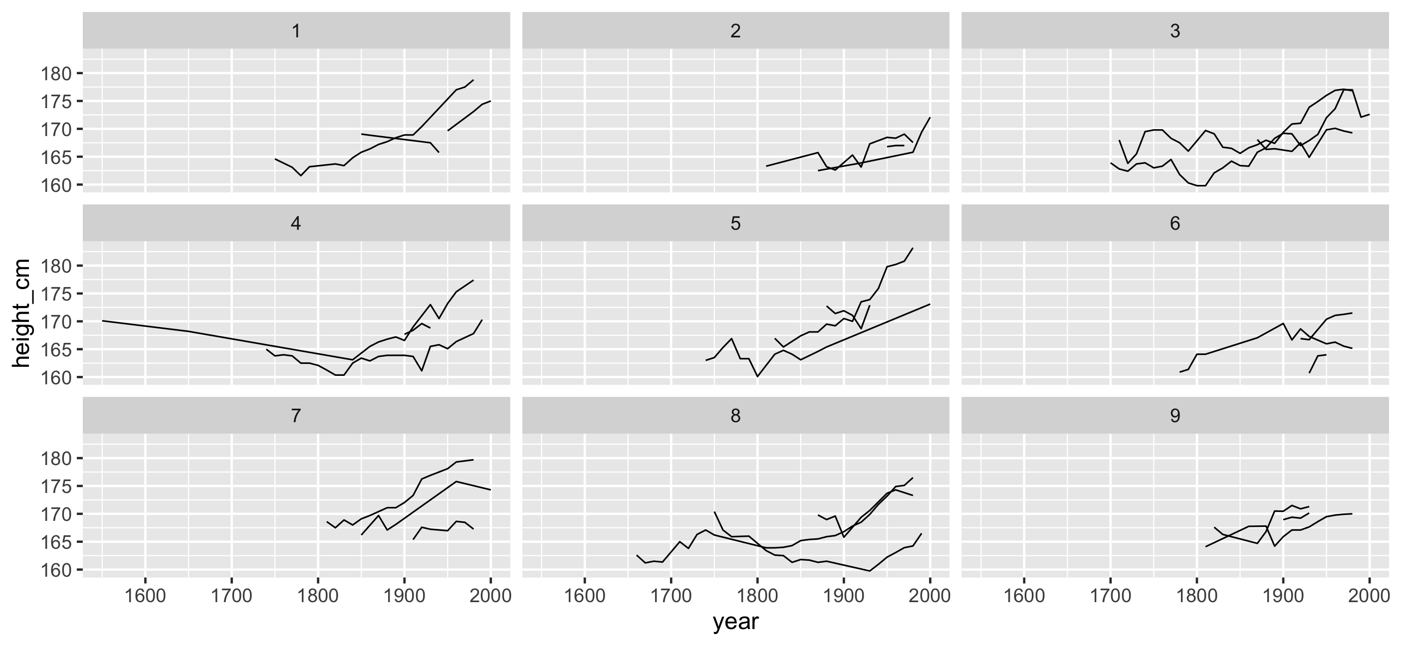
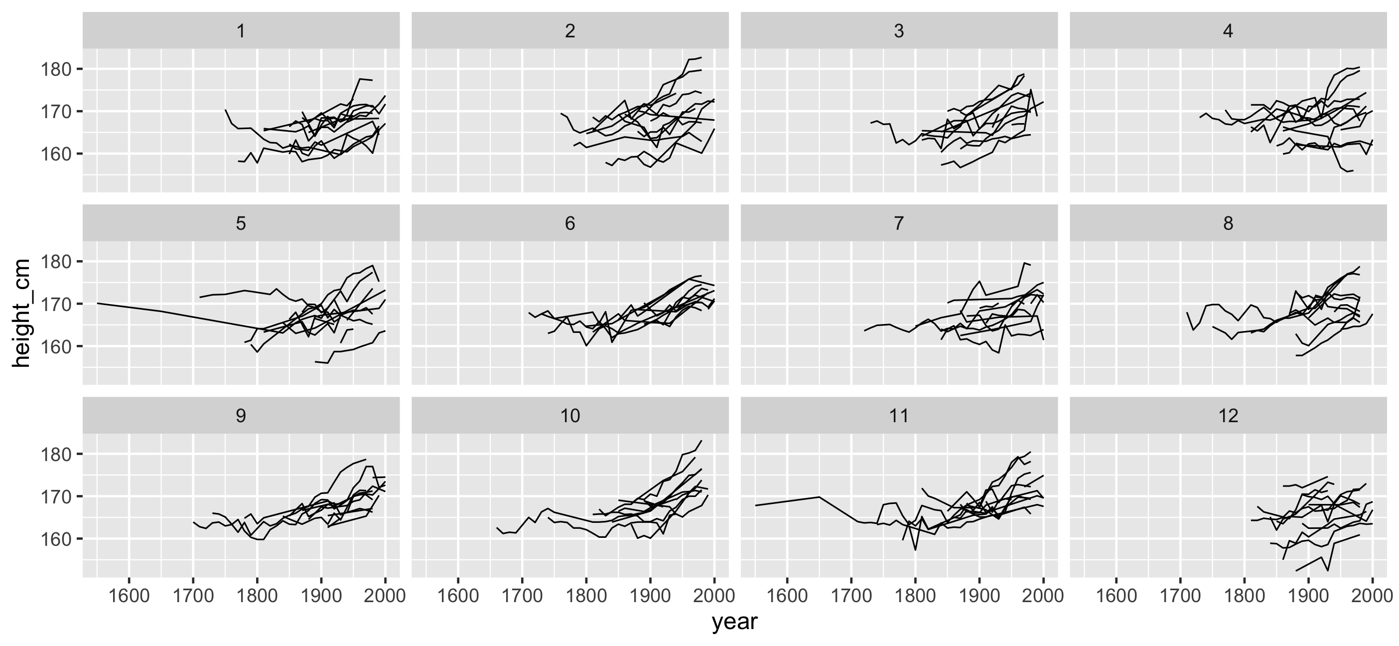
facet_strata(): See all individuals
Can we re-order these facets in a meaningful way?
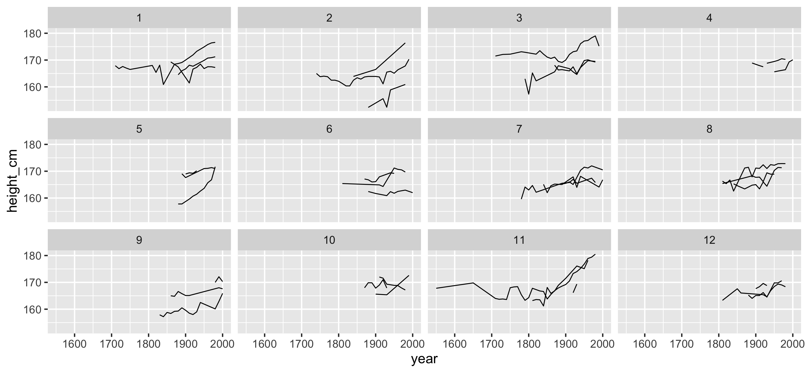
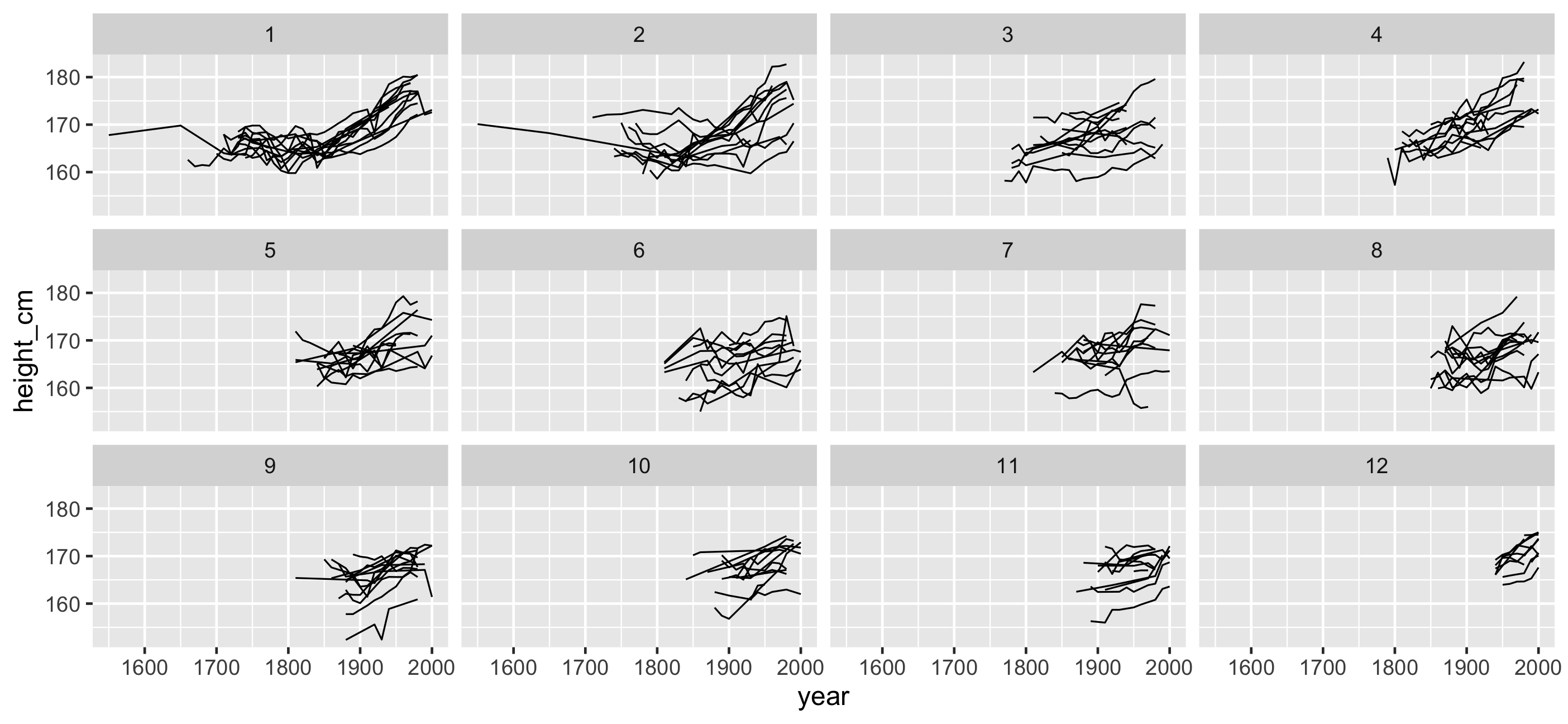
facet_strata(along = -year): see all individuals along some variable
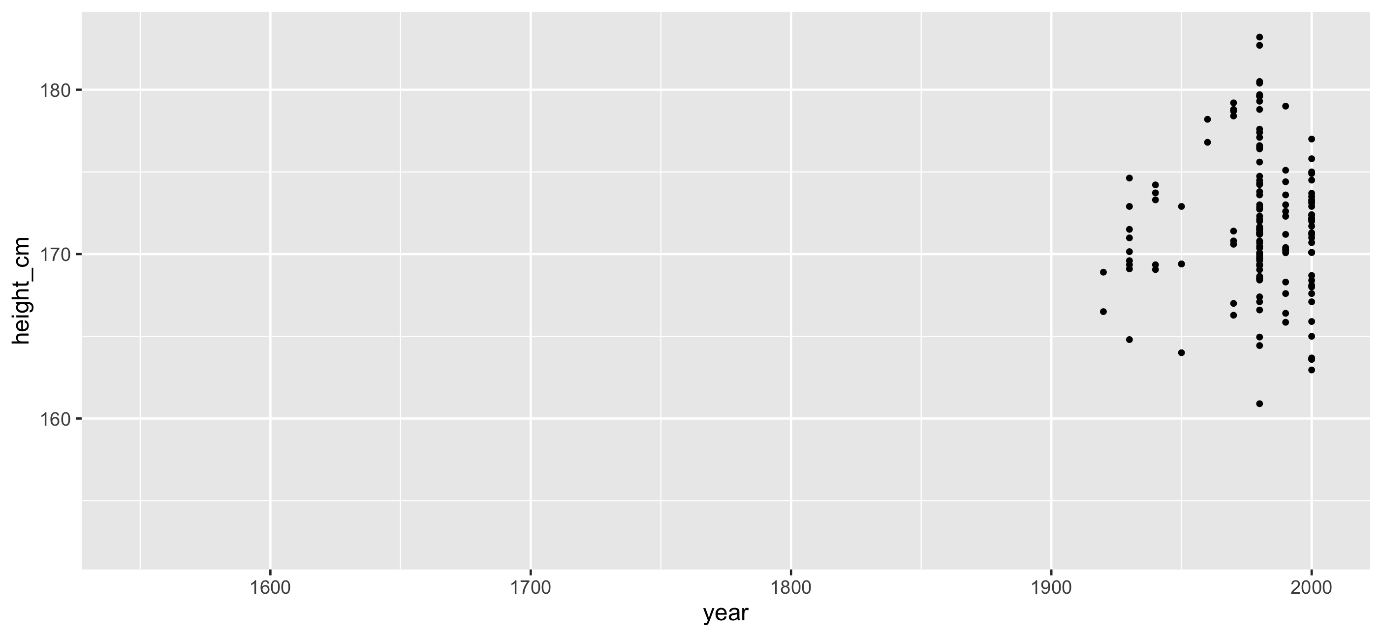
Problem #2: How do I find interesting observations?
Identify features: one observation per key

Identify features: one observation per key
Identify features: one observation per key
Identify important features and decide how to filter
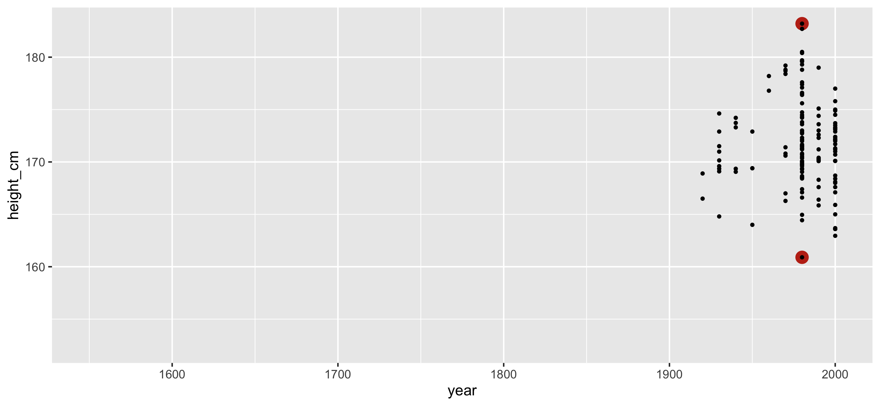
Identify important features and decide how to filter
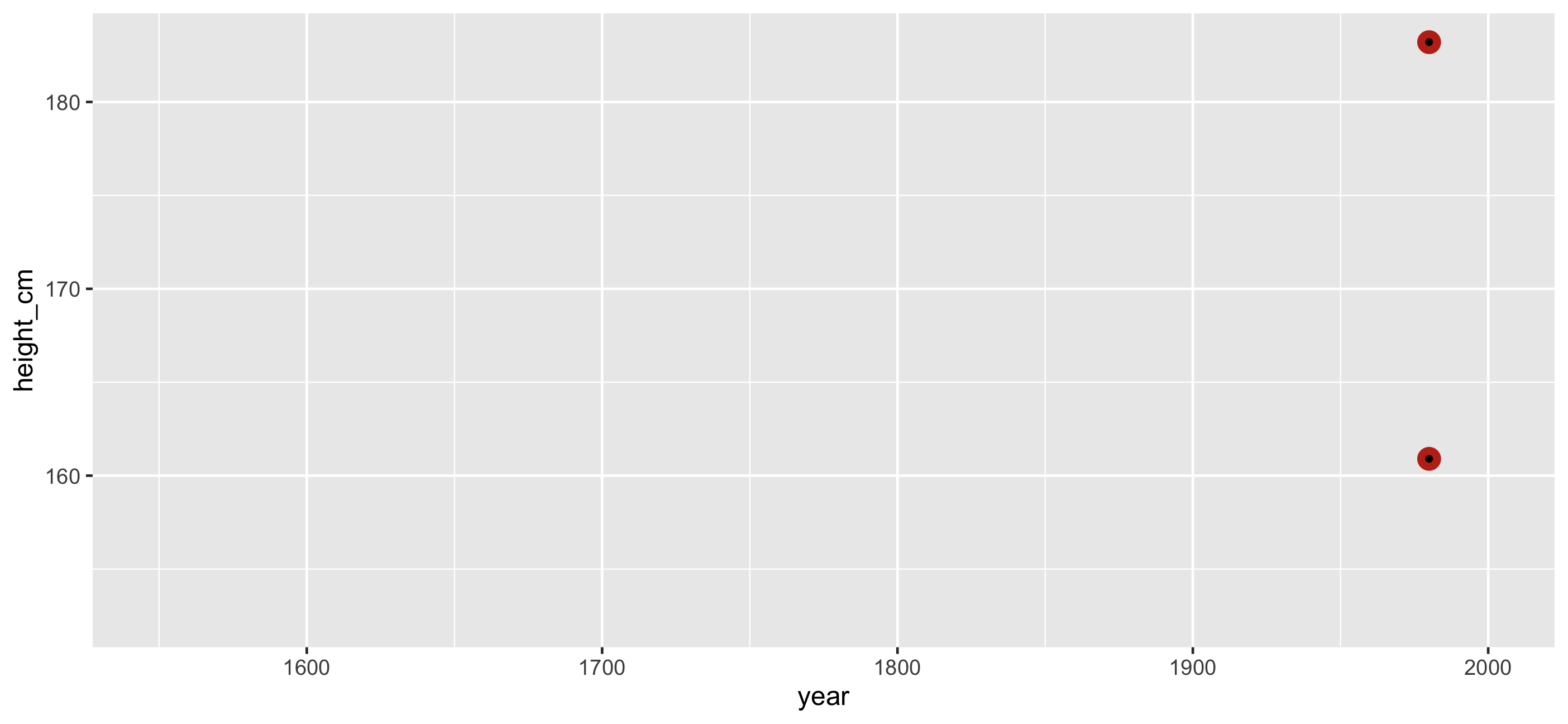
Join this feature back to the data
Join this feature back to the data
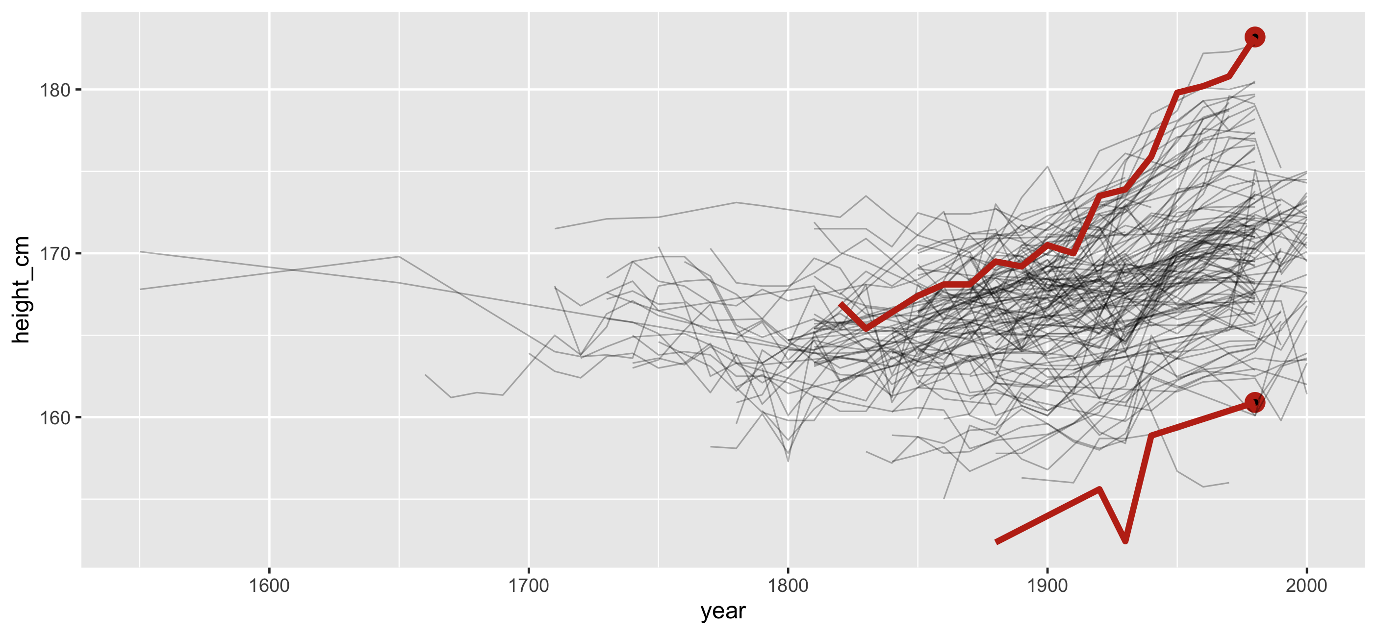
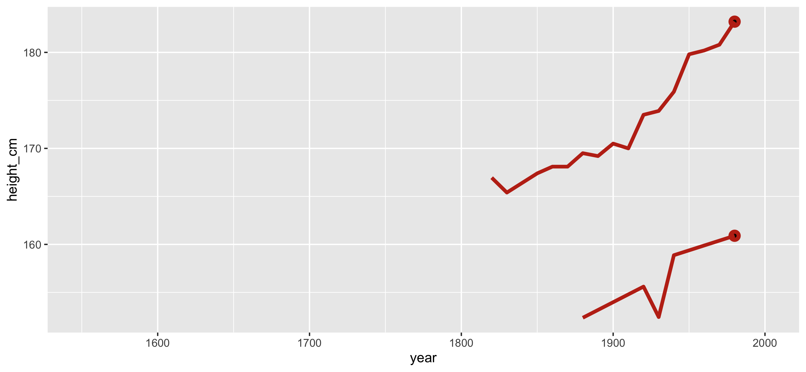
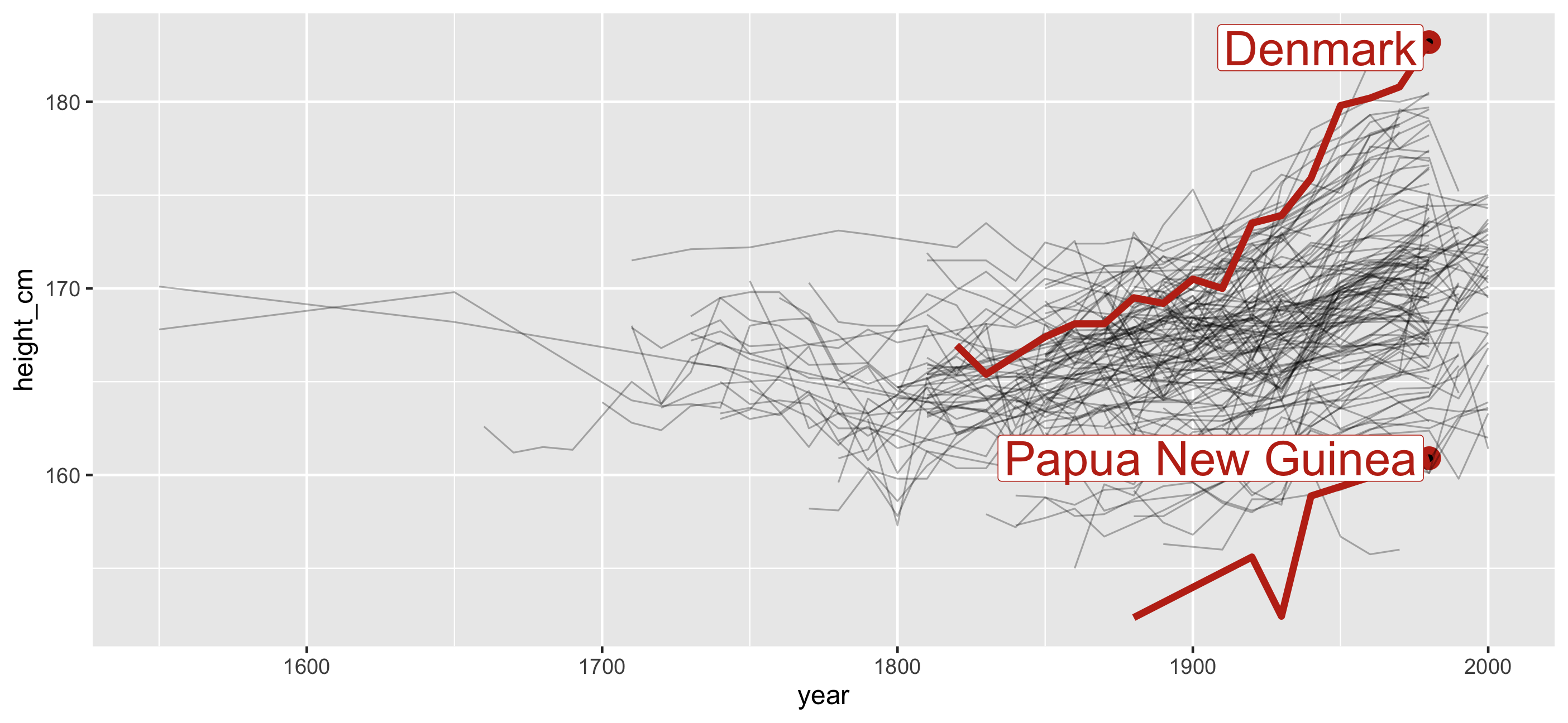
🎉 Countries with smallest and largest max height
Identify features: one per key 
heights %>% features(height_cm, feat_five_num)## # A tibble: 144 x 6## country min q25 med q75 max## <chr> <dbl> <dbl> <dbl> <dbl> <dbl>## 1 Afghanistan 161. 164. 167. 168. 168.## 2 Albania 168. 168. 170. 170. 170.## 3 Algeria 166. 168. 169 170. 171.## 4 Angola 159. 160. 167. 168. 169.## 5 Argentina 167. 168. 168. 170. 174.## 6 Armenia 164. 166. 169. 172. 172.## # … with 138 more rowsfeatures: MANY more features in feasts
Such as:
feat_acf: autocorrelation-based featuresfeat_stl: STL (Seasonal, Trend, and Remainder by LOESS) decomposition- Create your own features